Walkthrough

size, bs = 128, 32
dls = get_dls(size, bs)

Let’s start with a bit of context for the purpose of the demonstration. Imagine that we want to deploy a VGG16 model on a mobile device that has limited storage capacity and that our task requires our model to run sufficiently fast. It is known that parameters and speed efficiency are not the strong points of VGG16 but let’s see what we can do with it.

Let’s first check the number of parameters and the inference time of VGG16.

learn = Learner(dls, models.vgg16_bn(num_classes=10), metrics=[accuracy])

So, VGG16 has 134 millions of parameters

count_parameters(learn.model)

Total parameters : 134,309,962

And takes 28ms to perform inference on a single image.

model = learn.model.eval().to('cpu')
x,y = dls.one_batch()

model(x[0][None].to('cpu'))

27.9 ms ± 431 µs per loop (mean ± std. dev. of 7 runs, 10 loops each)

Snap ! This is more than we can afford for deployment, ideally we would like our model to take only half of that…but should we give up ? Nope, there are actually a lot of techniques that we can use to help reducing the size and improve the speed of our models! Let’s see how to apply them with FasterAI.

We will first train our VGG16 model to have a baseline of what performance we should expect from it.

learn.fit_one_cycle(10, 1e-4)

epoch	train_loss	valid_loss	accuracy	time
0	2.099871	1.795673	0.387771	00:27
1	1.710326	1.525811	0.497580	00:26
2	1.436516	1.337613	0.565096	00:26
3	1.215660	1.325269	0.573758	00:26
4	1.039825	0.970052	0.695287	00:26
5	0.891981	0.940327	0.710318	00:26
6	0.866332	0.760897	0.762803	00:26
7	0.729261	0.625635	0.795414	00:26
8	0.621271	0.584773	0.810701	00:26
9	0.608381	0.590041	0.808917	00:27

So we would like our network to have comparable accuracy but fewer parameters and running faster… And the first technique that we will show how to use is called Knowledge Distillation

Knowledge Distillation

Knowledge distillation is a simple yet very efficient way to train a model. It was introduced in 2006 by Caruana et al.. The main idea behind is to use a small model (called the student) to approximate the function learned by a larger and high-performing model (called the teacher). This can be done by using the large model to pseudo-label the data. This idea has been used very recently to break the state-of-the-art accuracy on ImageNet.

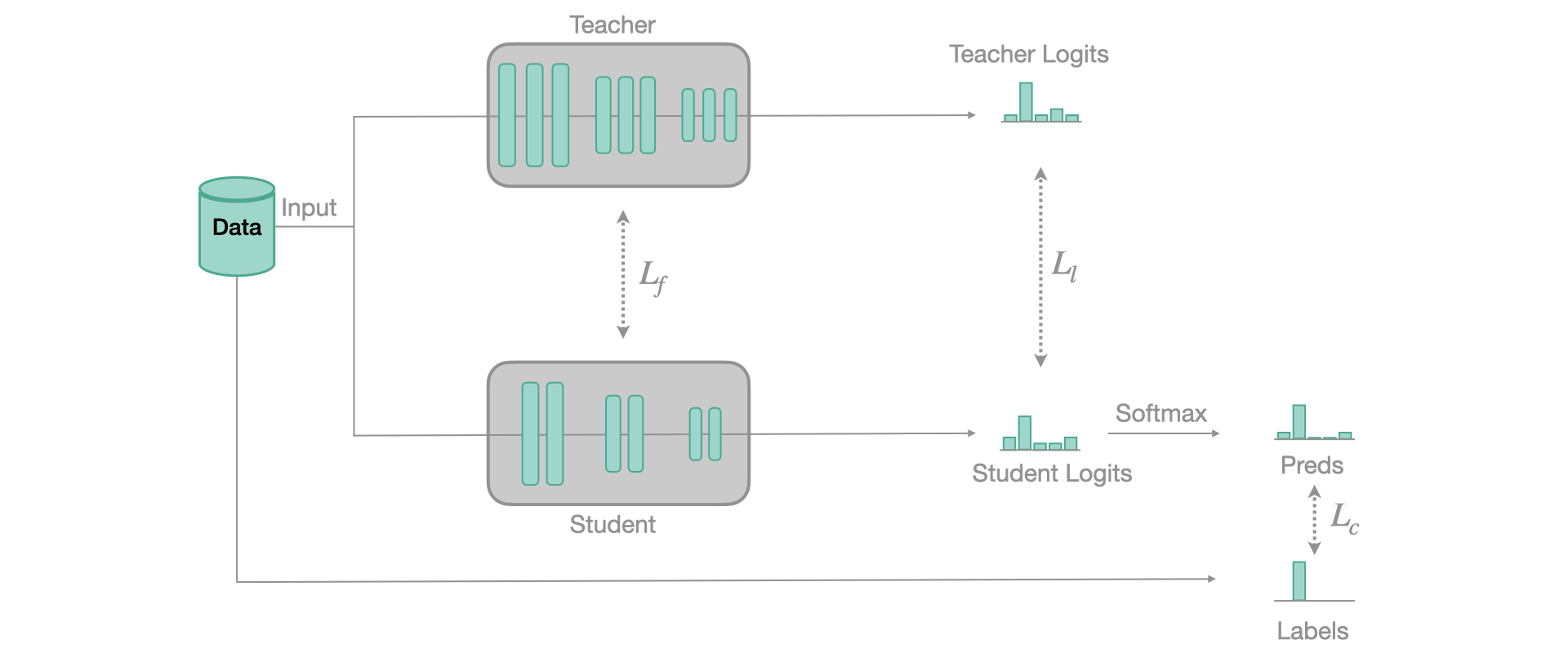
When we train our model for classification, we usually use a softmax as last layer. This softmax has the particularity to squish low value logits towards 0, and the highest logit towards 1. This has for effect to completely lose all the inter-class information, or what is sometimes called the dark knowledge. This is the information that is valuable and that we want to transfer from the teacher to the student.

To do so, we still use a regular classification loss but at the same time, we’ll use another loss, computed between the softened logits of the teacher (our soft labels) and the softened logits of the student (our soft predictions). Those soft values are obtained when you use a soft-softmax, that avoids squishing the values at its output. Our implementation follows this paper and the basic principle of training is represented in the figure below:

To use Knowledge Distillation with FasterAI, you only need to use this callback when training your student model:

 KnowledgeDistillation(teacher.model, loss) 
You only need to give to the callback function your teacher learner. Behind the scenes, FasterAI will take care of making your model train using knowledge distillation.

from fasterai.distill.all import *

The first thing to do is to find a teacher, which can be any model, that preferrably performs well. We will chose VGG19 for our demonstration. To make sure it performs better than our VGG16 model, let’s start from a pretrained version.

teacher = vision_learner(dls, models.vgg19_bn, metrics=[accuracy])
teacher.fit_one_cycle(3, 1e-4)

epoch	train_loss	valid_loss	accuracy	time
0	0.935599	0.368946	0.887898	00:18
1	0.428204	0.229474	0.928662	00:18
2	0.400993	0.204291	0.936051	00:19

Our teacher has 94% of accuracy which is pretty good, it is ready to take a student under its wing. So let’s create our student model and train it with the Knowledge Distillation callback:

student = Learner(dls, models.vgg16_bn(num_classes=10), metrics=[accuracy])
kd_cb = KnowledgeDistillationCallback(teacher.model, SoftTarget)
student.fit_one_cycle(10, 1e-4, cbs=kd_cb)

epoch	train_loss	valid_loss	accuracy	time
0	6.307211	5.839308	0.347006	00:43
1	4.398540	4.453655	0.534777	00:43
2	3.618300	3.845923	0.588535	00:43
3	3.301258	3.164423	0.649936	00:43
4	2.803221	2.299710	0.740382	00:43
5	2.378756	2.147169	0.755924	00:43
6	2.118665	2.143216	0.781911	00:43
7	1.814469	1.728230	0.802293	00:43
8	1.686883	1.566467	0.831592	00:43
9	1.650822	1.547276	0.828280	00:43

And we can see that indeed, the knowledge of the teacher was useful for the student, as it is clearly overperforming the vanilla VGG16.

Ok, so now we are able to get more from a given model which is kind of cool ! With some experimentations we could come up with a model smaller than VGG16 but able to reach the same performance as our baseline! You can try to find it by yourself later, but for now let’s continue with the next technique !

Sparsifying

Now that we have a student model that is performing better than our baseline, we have some room to compress it. And we’ll start by making the network sparse. As explained in a previous article, there are many ways leading to a sparse network.

Note

Usually, the process of making a network sparse is called Pruning. I prefer using the term Pruning when parameters are actually removed from the network, which we will do in the next section.

By default, FasterAI uses the Automated Gradual Pruning paradigm as it removes parameters as the model trains and doesn’t require to pretrain the model, so it is usually much faster. In FasterAI, this is also managed by using a callback, that will replace the least important parameters of your model by zeroes during the training. The callback has a wide variety of parameters to tune your Sparsifying operation, let’s take a look at them:

SparsifyCallback(learn, sparsity, granularity, context, criteria, schedule)
sparsity: the percentage of sparsity that you want in your network

granularity: on what granularity you want the sparsification to be operated

context: either local or global, will affect the selection of parameters to be choosen in each layer independently (local) or on the whole network (global).

criteria: the criteria used to select which parameters to remove (currently supported: l1, taylor)

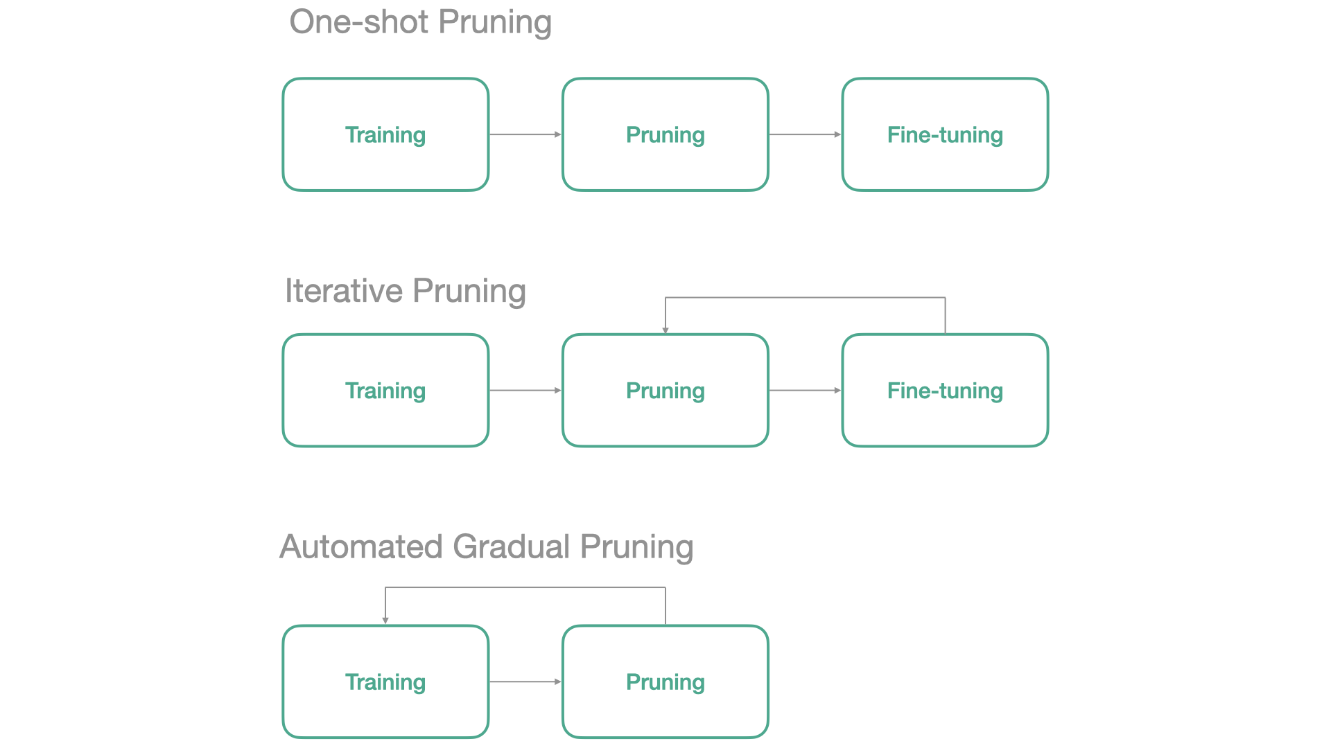
schedule: which schedule you want to follow for the sparsification (currently supported: any scheduling function of fastai, i.e linear, cosine, … and gradual, common schedules such as One-Shot, Iterative or Automated Gradual)

But let’s come back to our example!

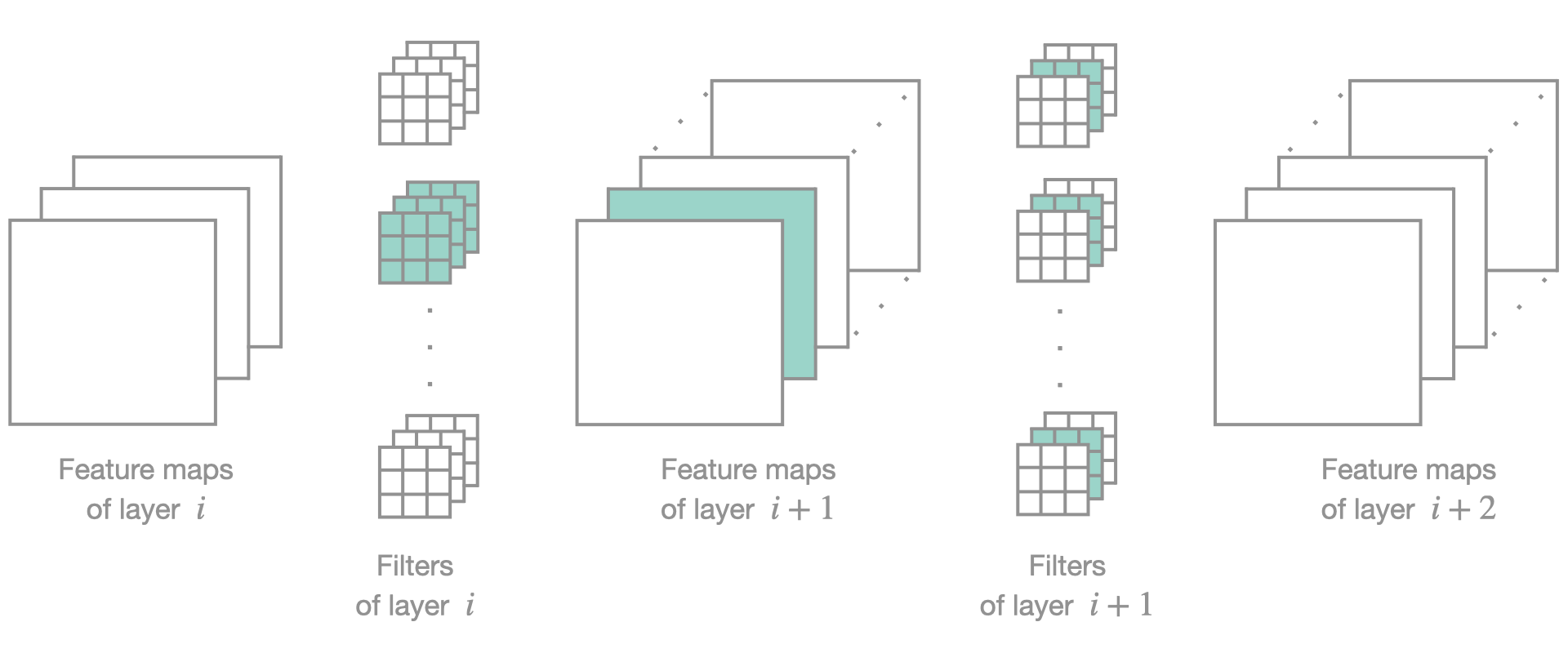
Here, we will make our network 40% sparse, and remove entire filters, selected locally and based on L1 norm. We will train with a learning rate a bit smaller to be gentle with our network because it has already been trained. The scheduling selected is cosinusoidal, so the pruning starts and ends quite slowly.

sp_cb = SparsifyCallback(sparsity=50, granularity='filter', context='global', criteria=large_final, schedule=cos)
student.fit(10, 1e-5, cbs=sp_cb)

Pruning of filter until a sparsity of [50]%
Saving Weights at epoch 0
Sparsity at the end of epoch 0: [1.22]%
Sparsity at the end of epoch 1: [4.77]%
Sparsity at the end of epoch 2: [10.31]%
Sparsity at the end of epoch 3: [17.27]%
Sparsity at the end of epoch 4: [25.0]%
Sparsity at the end of epoch 5: [32.73]%
Sparsity at the end of epoch 6: [39.69]%
Sparsity at the end of epoch 7: [45.23]%
Sparsity at the end of epoch 8: [48.78]%
Sparsity at the end of epoch 9: [50.0]%
Final Sparsity: [50.0]%
Sparsity in Conv2d 2: 0.00%
Sparsity in Conv2d 5: 0.00%
Sparsity in Conv2d 9: 0.00%
Sparsity in Conv2d 12: 0.00%
Sparsity in Conv2d 16: 0.00%
Sparsity in Conv2d 19: 0.00%
Sparsity in Conv2d 22: 0.00%
Sparsity in Conv2d 26: 65.04%
Sparsity in Conv2d 29: 72.66%
Sparsity in Conv2d 32: 72.85%
Sparsity in Conv2d 36: 66.41%
Sparsity in Conv2d 39: 67.58%
Sparsity in Conv2d 42: 67.97%

epoch	train_loss	valid_loss	accuracy	time
0	0.575622	0.552721	0.830064	00:27
1	0.547505	0.547928	0.827771	00:27
2	0.534454	0.538333	0.831338	00:27
3	0.600492	0.549522	0.827771	00:27
4	0.582688	0.547946	0.825732	00:27
5	0.589183	0.570673	0.816561	00:27
6	0.585249	0.595492	0.811465	00:27
7	0.599623	0.612489	0.801019	00:27
8	0.617754	0.621315	0.796943	00:27
9	0.614237	0.609054	0.797962	00:27

Our network now has 50% of its filters composed entirely of zeroes, without even losing accuracy. Obviously, choosing a higher sparsity makes it more difficult for the network to keep a similar accuracy. Other parameters can also widely change the behaviour of our sparsification process. For example choosing a more fine-grained sparsity usually leads to better results but is then more difficult to take advantage of in terms of speed.

Let’s now see how much we gained in terms of speed. Because we removed 50% of convolution filters, we should expect crazy speed-up right ?

model = student.model.eval().to('cpu')

model(x[0][None].to('cpu'))

26.8 ms ± 22.6 µs per loop (mean ± std. dev. of 7 runs, 10 loops each)

Well actually, no. We didn’t remove any parameters, we just replaced some by zeroes, remember? The amount of parameters is still the same:

count_parameters(model)

Total parameters : 134,309,962

Which leads us to the next section.

Pruning

Why don’t we see any acceleration even though we removed half of the parameters? That’s because natively, our GPU does not know that our matrices are sparse and thus isn’t able to accelerate the computation. The easiest work around, is to physically remove the parameters we zeroed-out. But this operation requires to change the architecture of the network.

This pruning only works if we remove entire filters as it is the only case where we can change the architecture accordingly. Hopefully, sparse computations will soon be available on common deep learning librairies so this section will become useless in the future.

Here is what it looks like with fasterai:

PruneCallback(learn, sparsity, context, criteria, schedule)
sparsity: the percentage of sparsity that you want in your network

context: either local or global, will affect the selection of parameters to be choosen in each layer independently (local) or on the whole network (global).

criteria: the criteria used to select which parameters to remove (currently supported: l1, taylor)

schedule: which schedule you want to follow for the sparsification (currently supported: any scheduling function of fastai, i.e linear, cosine, … and gradual, common schedules such as One-Shot, Iterative or Automated Gradual)

So in the case of our example, it gives:

from fasterai.prune.all import *

Let’s now see what our model is capable of now:

pr_cb = PruneCallback(sparsity=50, context='global', criteria=large_final, schedule=cos, layer_type=[nn.Conv2d])
student.fit(5, 1e-5, cbs=pr_cb)

Pruning until a sparsity of [50]%
Sparsity at the end of epoch 0: [4.77]%
Sparsity at the end of epoch 1: [17.27]%
Sparsity at the end of epoch 2: [32.73]%
Sparsity at the end of epoch 3: [45.23]%
Sparsity at the end of epoch 4: [50.0]%
Final Sparsity: [50.0]%

epoch	train_loss	valid_loss	accuracy	time
0	0.565141	0.577327	0.810955	01:25
1	0.568069	0.585159	0.809172	00:59
2	0.580409	0.576743	0.814013	00:47
3	0.511273	0.572584	0.811975	00:46
4	0.546116	0.576101	0.812229	00:45

count_parameters(student.model)

Total parameters : 54,621,297

And in terms of speed:

model = student.model.eval().to('cpu')

model(x[0][None].to('cpu'))

16.6 ms ± 562 µs per loop (mean ± std. dev. of 7 runs, 100 loops each)

Yay ! Now we can talk ! Let’s just double check that our accuracy is unchanged and that we didn’t mess up somewhere:

And there is actually more that we can do ! Let’s keep going !

Batch Normalization Folding

Batch Normalization Folding is a really easy to implement and straightforward idea. The gist is that batch normalization is nothing more than a normalization of the input data at each layer. Moreover, at inference time, the batch statistics used for this normalization are fixed. We can thus incorporate the normalization process directly in the convolution by changing its weights and completely remove the batch normalization layers, which is a gain both in terms of parameters and in terms of computations. For a more in-depth explaination, see this blog post.

This is how to use it with FasterAI:

bn_folder = BN_Folder()
bn_folder.fold(learn.model))
Again, you only need to pass your model and FasterAI takes care of the rest. For models built using the nn.Sequential, you don’t need to change anything. For others, if you want to see speedup and compression, you actually need to subclass your model to remove the batch norm from the parameters and from the forward method of your network.

Note

This operation should also be lossless as it redefines the convolution to take batch norm into account and is thus equivalent.

from fasterai.misc.bn_folding import *

Let’s do this with our model !

bn_f = BN_Folder()
folded_model = bn_f.fold(student.model)

The parameters drop is generally not that significant, especially in a network such as VGG where almost all parameters are contained in the FC layers but, hey, any gain is good to take.

count_parameters(folded_model)

Total parameters : 54,617,073

Now that we removed the batch normalization layers, we should again see a speedup.

folded_model = folded_model.eval().to('cpu')

folded_model(x[0][None].to('cpu'))

15.5 ms ± 10.3 µs per loop (mean ± std. dev. of 7 runs, 100 loops each)

Again, let’s double check that we didn’t mess up somewhere:

folded_learner = Learner(dls, folded_model, metrics=[accuracy])
folded_learner.validate()

(#2) [0.5759302973747253,0.8119745254516602]

And we’re still not done yet ! As we know for VGG16, most of the parameters are comprised in the fully-connected layers so there should be something that we can do about it, right ?

FC Layers Factorization

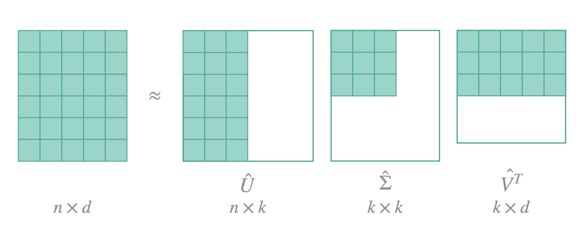
We can indeed, factorize our big fully-connected layers and replace them by an approximation of two smaller layers. The idea is to make an SVD decomposition of the weight matrix, which will express the original matrix in a product of 3 matrices: \(U \Sigma V^T\). With \(\Sigma\) being a diagonal matrix with non-negative values along its diagonal (the singular values). We then define a value \(k\) of singular values to keep and modify matrices \(U\) and \(V^T\) accordingly. The resulting will be an approximation of the initial matrix.

In FasterAI, to decompose the fully-connected layers of your model, here is what you need to do:

FCD = FCDecomposer()
decomposed_model = FCD.decompose(model, percent_removed)
The percent_removed corresponds to the percentage of singular values removed (k value above).

Note

This time, the decomposition is not exact, so we expect a drop in performance afterwards and further retraining will be needed.

Which gives with our example, if we only want to keep half of them:

from fasterai.misc.fc_decomposer import *

fc_decomposer = FC_Decomposer()
decomposed_model = fc_decomposer.decompose(folded_model, percent_removed=0.5)

How many parameters do we have now ?

count_parameters(decomposed_model)

Total parameters : 45,724,707

And how much time did we gain ?

decomposed_model = decomposed_model.eval().to('cpu')

decomposed_model(x[0][None].to('cpu'))

14.8 ms ± 19.7 µs per loop (mean ± std. dev. of 7 runs, 100 loops each)

We actually get a network that is a little bit slower, but at the expense of reducing the by 10M the number of parameter. This is thus a matter of compromise between network weight and speed.

However, this technique is an approximation so it is not lossless, so we should retrain our network a bit to recover its performance.

final_learner = Learner(dls, decomposed_model, metrics=[accuracy])
final_learner.fit_one_cycle(5, 1e-5)

epoch	train_loss	valid_loss	accuracy	time
0	0.893666	0.865394	0.729682	00:17
1	0.766977	0.834168	0.749299	00:17
2	0.693381	0.715239	0.799236	00:17
3	0.629866	0.700622	0.796433	00:17
4	0.614129	0.669185	0.806624	00:17

This operation is usually less useful for more recent architectures as they usually do not have that many parameters in their fully-connected layers.

Quantization

from fasterai.quantize.quantize_callback import *

final_learner.fit_one_cycle(5, 1e-5, cbs=QuantizeCallback())

epoch	train_loss	valid_loss	accuracy	time
0	0.675018	0.728861	0.790828	00:23
1	0.672481	0.717207	0.795159	00:23
2	0.590282	0.647120	0.809427	00:23
3	0.553525	0.645101	0.811465	00:23
4	0.525336	0.640611	0.815032	00:23

final_learner.model(x[0][None].to('cpu'))

12.2 ms ± 5.27 µs per loop (mean ± std. dev. of 7 runs, 100 loops each)

count_parameters_quantized(final_learner.model)

Total parameters: 45,724,707

So to recap, we saw in this article how to use fasterai to:
1. Make a student model learn from a teacher model (Knowledge Distillation)
2. Make our network sparse (Sparsifying)
3. Optionnaly physically remove the zero-filters (Pruning)
4. Remove the batch norm layers (Batch Normalization Folding)
5. Approximate our big fully-connected layers by smaller ones (Fully-Connected Layers Factorization)
6. Quantize the model to reduce the precision of the weights (Quantization)

And we saw that by applying those, we could reduce our VGG16 model from 134 million of parameters down to 45 million, and also speed-up the inference from 26ms to 12ms without any drop in accuracy compared to the baseline.

Note

Please keep in mind that the techniques presented above are not magic 🧙‍♂️, so do not expect to see a 200% speedup and compression everytime. What you can achieve highly depend on the architecture that you are using (some are already speed/parameter efficient by design) or the task it is doing (some datasets are so easy that you can remove almost all your network without seeing a drop in performance)